Posts so far in this blog have focused on creating web maps with vector tiles i.e. maps made up of point, line, and polygon geometries, rendered client side in a browser. Alternatively, a web map can be pre-rendered and served using raster tiles (i.e. images), as is often done by many web map providers, including OpenStreetMap (OSM).
Raster tiles can be a good choice for a basemap when the styling is intended to be static i.e. rarely updated, and non-interactive. They can potentially allow for a greater level of detail, as being pre-rendered, they are not affected by the geometry simplification or feature limits required by vector tiles for client side rendering.
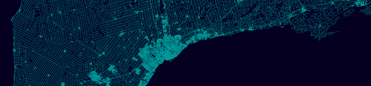
This post details a workflow for creating a custom styled OSM raster map of Ontario, utilizing elements of the openmaptiles stack for data processing, and tilemill for map styling, replicating the basemap below:
OSM import
To get started, first download the ontario-latest OSM database from geofabrik in .osm.pbf format. The PBF format used by OSM is highly compressed and contains many, many tags (attributes), and so requires processing to extract the features and attributes of interest. In this case we will use Imposm to filter and transform the PBF file to a PostGIS spatial database.
First start a PostGIS database with Docker:
docker pull openmaptiles/postgis

docker run \
     -d \
     --name=osm-db \
     -v $(PWD)/pg-data:/var/lib/postgresql/data \
     -e POSTGRES_DB="osm" \
     -e POSTGRES_USER="mapping-on" \
     -e POSTGRES_PASSWORD="mapping-on" \
     openmaptiles/postgis
Next, download an example of the mapping file that Imposm will use to filter the OSM layers and tags and create database tables. Save this to the same directory as the OSM PBF file and then run the import container. Note that on my machine, this process took around an hour to complete.
docker pull openmaptiles/import-osm

docker run \
     --rm \
     -v $(PWD)/ontario-latest.osm.pbf:/import/ontario-latest.osm.pbf \
     -v $(PWD)/example-mapping.yml:/mapping/mapping.yaml \
     -e POSTGRES_USER="mapping-on" \
     -e POSTGRES_PASSWORD="mapping-on" \
     -e POSTGRES_HOST="localhost" \
     -e POSTGRES_DB="osm" \
     -e POSTGRES_PORT="5432" \
     openmaptiles/import-osm
Tilemill project setup
Once the import has completed, we can start a tilemill container for designing the map as below. You then connect to the tilemill interface in a browser at localhost:20009, although it may take a few minutes before you can connect, while the app starts up.
docker pull hansmeine/tilemill

docker run \
     -d \
     -t \
     --name tilemill \
     -v $(PWD)/tilemill:/root/Documents/MapBox \
     -p 20009:20009 \
     -p 20008:20008 \
     hansmeine/tilemill:latest
Within the tilemill app, select New project, and enter a suitable Filename and Name for the project, and optionally a Description, then click Add to start the project.

A default countries layer is included with the map style, which we will extend with some of the layers imported to our OSM database. To do so, click the layers icon ![]() and select Add Layer. In this form, we will enter the connection details for your database, and specify the SQL for selecting the target layer and columns, for example the osm_waterareas_gen0 layer:
and select Add Layer. In this form, we will enter the connection details for your database, and specify the SQL for selecting the target layer and columns, for example the osm_waterareas_gen0 layer:

Breaking this down, this form should be completed with the following main details:
ID: The unique name to refer to the layer for styling e.g. osm-waterareas-gen0
Connection: The connection string for your database e.g. host=database container ip dbname=osm user=mapping-on password=mapping-on port=5432
Table or subquery: The SQL query e.g. select st_area(geometry) as area, geometry from osm_waterareas_gen0 where type in (‘water’, ‘reservoir’)
To get your Docker database container ip address to use for the connection string host parameter, enter the below command in a terminal and look for the “IPv4Address” for your “osm-db” container. The host is this value, excluding the slash and anything after it.
docker network inspect bridge
Once complete, click Save, and then repeat the process for the remaining layers, using the same connection string, but setting the ID and SQL queries as per the table below. This will add layers for water polygons (waterareas), waterways, and roads at three different levels of detail, plus layers with administration boundaries and place names.
| ID | Table or subquery |
| osm-waterareas-gen1 | select geometry from osm_waterareas_gen1 where type in (‘water’, ‘reservoir’) |
| osm-waterareas | select geometry from osm_waterareas where type in (‘water’, ‘reservoir’) |
| osm-waterways-gen0 | select geometry from osm_waterways_gen0 |
| osm-waterways-gen1 | select geometry from osm_waterways_gen1 |
| osm-waterways | select geometry from osm_waterways |
| osm-roads | select type, geometry from osm_roads where type in (‘motorway’, ‘tertiary’, ‘trunk’, ‘tertiary_link’, ‘motorway_link’, ‘secondary_link’, ‘primary_link’, ‘trunk_link’, ‘road’, ‘secondary’, ‘primary’) |
| osm-roads-gen0 | select type, geometry from osm_roads_gen0 where type in (‘motorway’, ‘tertiary’, ‘trunk’, ‘tertiary_link’, ‘motorway_link’, ‘secondary_link’, ‘primary_link’, ‘trunk_link’, ‘road’, ‘secondary’, ‘primary’) |
| osm-roads-gen1 | select type, geometry from osm_roads_gen1 where type in (‘motorway’, ‘tertiary’, ‘trunk’, ‘tertiary_link’, ‘motorway_link’, ‘secondary_link’, ‘primary_link’, ‘trunk_link’, ‘road’, ‘secondary’, ‘primary’) |
| osm-roads | select type, geometry from osm_roads where type in (‘motorway’, ‘tertiary’, ‘trunk’, ‘tertiary_link’, ‘motorway_link’, ‘secondary_link’, ‘primary_link’, ‘trunk_link’, ‘road’, ‘secondary’, ‘primary’) |
| osm-admin | select geometry from osm_admin where admin_level = 4 |
| osm-places | select name, type, population, geometry from osm_places where type in (‘town’, ‘city’, ‘village’) order by population desc |
Styling
With all layers added to the map, it is time to style them by editing the style.mss file in the editor on the right side of the app, copying and pasting the styling for each layer from the example below.
@water: #DCDCDC;
@roads: #C0C0C0;
@admin: #A9A9A9;
@sans-bold:"Arial Bold","Liberation Sans Bold","DejaVu Sans Bold";

Map {
  background-color: @water;
}

#countries {
  polygon-fill: #fff;
}

#admin-level {
  line-color: @admin;
  line-width: 2;
  polygon-opacity: 0;
}

#osm-waterways [zoom > 10] {
  line-width: 1;
  line-color: @water;
}

#osm-waterways-gen1 [zoom = 10] {
  line-width: 1;
  line-color: @water;
}

#osm-waterways-gen0 [zoom = 9] {
  line-width: 1;
  line-color: @water;
}

#osm-waterways-gen0 [zoom = 8] {
  line-width: 0.5;
  line-color: @water;
}

#osm-waterareas [zoom > 10] {
  polygon-fill: @water;
}

#osm-waterareas-gen1 [zoom = 10] {
  polygon-fill: @water;
}

#osm-waterareas-gen0 [zoom >= 8][zoom < 10] {
  polygon-fill: @water;
}

#osm-waterareas-gen0 [zoom = 7][area > 1000000] {
  polygon-fill: @water;
}

#osm-waterareas-gen0 [zoom = 6][area > 10000000] {
  polygon-fill: @water;
}

#osm-waterareas-gen0 [zoom = 5][area > 50000000] {
  polygon-fill: @water;
}

#osm-roads [zoom > 10] {
  line-width: 0.5;
  line-color: @roads;
  [type ='motorway'],[type = 'trunk'],[type = 'motorway_link'],[type = 'secondary_link'],[type = 'primary_link'],[type = 'trunk_link'],[type = 'secondary'],[type = 'primary'] {
    line-width: 1;
   }
}

#osm-roads-gen1 [zoom = 10] {
  line-width: 0.5;
  line-color: @roads;
  [type ='motorway'],[type = 'trunk'],[type = 'motorway_link'],[type = 'secondary_link'],[type = 'primary_link'],[type = 'trunk_link'],[type = 'secondary'],[type = 'primary'] {
    line-width: 1;
   }
}

#osm-roads-gen0 [zoom >= 8][zoom < 10] {
  line-width: 0.5;
  line-color: @roads;
  [type ='motorway'],[type = 'trunk'],[type = 'motorway_link'],[type = 'secondary_link'],[type = 'primary_link'],[type = 'trunk_link'],[type = 'secondary'],[type = 'primary'] {
    line-width: 1;
   }
}

#osm-roads-gen0 [zoom = 7] {
  [type ='motorway'],[type = 'trunk'],[type = 'motorway_link'],[type = 'secondary_link'],[type = 'primary_link'],[type = 'trunk_link'],[type = 'secondary'],[type = 'primary'] {
    line-width: 0.5;
    line-width: 0.5;
    line-color: @roads;
  }
}

#osm-roads-gen0 [zoom = 6] {
  [type ='motorway'],[type = 'trunk'],[type = 'motorway_link'],[type = 'primary_link'],[type = 'trunk_link'],[type = 'primary'] {
    line-width: 0.5;
    line-width: 0.5;
    line-color: @roads;
  }
}

#osm-roads-gen0 [zoom = 5] {
  [type ='motorway'],[type = 'trunk'],[type = 'motorway_link'],[type = 'trunk_link'] {
    line-width: 0.5;
    line-width: 0.5;
    line-color: @roads;
  }
}

#osm-places [zoom >= 10][type = 'village'] {
  text-name:"[name]";
  text-face-name:@sans-bold;
  text-allow-overlap:false;
  text-character-spacing:1;
  text-line-spacing:4;
  text-size:8;
  text-wrap-width:120;
  text-allow-overlap:true;
  text-halo-radius:2;
  text-halo-fill:rgba(255,255,255,0.75);
  text-fill:darkgrey;
  text-min-distance: 30;
}

#osm-places [zoom >= 8][type = 'town'] {
  text-name:"[name]";
  text-face-name:@sans-bold;
  text-allow-overlap:false;
  text-character-spacing:1;
  text-line-spacing:4;
  text-size:8;
  text-wrap-width:120;
  text-allow-overlap:true;
  text-halo-radius:2;
  text-halo-fill:rgba(255,255,255,0.75);
  text-fill:darkgrey;
  text-min-distance: 30;
}

#osm-places [zoom >= 7][type = 'city'] {
  [population < 100000],[population = null] {
    text-name:"[name]";
    text-face-name:@sans-bold;
    text-allow-overlap:false;
    text-character-spacing:1;
    text-line-spacing:4;
    text-size:10;
    text-wrap-width:120;
    text-allow-overlap:true;
    text-halo-radius:2;
    text-halo-fill:rgba(255,255,255,0.75);
    text-fill:darkgrey;
    text-min-distance: 30;
  }
}

#osm-places [zoom >= 6][type = 'city'][population >= 100000][population < 500000] {
  text-name:"[name]";
  text-face-name:@sans-bold;
  text-allow-overlap:false;
  text-transform:uppercase;
  text-character-spacing:1;
  text-line-spacing:4;
  text-size:10;
  text-wrap-width:120;
  text-allow-overlap:true;
  text-halo-radius:2;
  text-halo-fill:rgba(255,255,255,0.75);
  text-fill:darkgrey;
  text-min-distance: 30;
}

#osm-places [zoom >= 5][type = 'city'][population >= 500000] {
  text-name:"[name]";
  text-face-name:@sans-bold;
  text-allow-overlap:false;
  text-transform:uppercase;
  text-character-spacing:1;
  text-line-spacing:4;
  text-size:12;
  text-wrap-width:120;
  text-allow-overlap:true;
  text-halo-radius:2;
  text-halo-fill:rgba(255,255,255,0.75);
  text-fill:darkgrey;
}
The styling language used for Tilemill is CartoCSS, which although outside the scope of this post to review in full, some features used in the style include:
- Referring to named parameters with @, here used to store and retrieve colour values.
- A “symbolizer” is defined with #, followed by the layer name and a pair of curly braces {}, within which are the styling details.
- Filtering for each individual symbolizer can be set with square braces [], which can include map parameters like zoom level, and layer column values like type.
- Styling is defined by providing values for various parameters, controlling things like colour, size, and text.
Export and serve
To export the map to raster tiles, select Export in the upper right of the application and choose MBTiles. In the export menu, set the Zoom levels to 5-13 and enter -96.41,-73.57 as the map Bounds to limit the number of tiles created, specify a Filename, then click Export, and once completed (which may take a while), save the mbtiles file locally.

The raster tiles can then be served with tileserver in a similar way to vector tiles in past posts e.g., in a terminal with the raster tiles saved in the current working directory, run a command like below.
docker run --rm -it -v $(pwd):/data -p 80:80 klokantech/tileserver-gl
Note that the tileserver app UI doesn’t present the correct urls, but the data is still being served, in this case the tiles url is at: http://localhost:80/data/osm-on/{z}/{x}/{y}.png8. An alternative could be to export the raster tiles to png files within directories with mbutil, which could then be served with nginx or similar.