A popular method for mapping census data is the “dot” density map, a method to randomly distribute values (often population counts) throughout geographic zones to visualize the variation in density across the zones. A well known example of such a map is The University of Virginia’s Racial Dot Map.
I recently posted my own version of a dot map, using Statistics Canada 2016 census data to map the speakers of Canada’s official languages of English and French (or both). This post details a similar method for creating a dot map table, implemented in Python 3 with libraries pandas and geopandas, and ran in an jupyter notebook as embedded below.
To run the code, download dissemination areas (Cartographic Boundary File) to use as the geographic zones, and a matching data table from the 2016 census – in this case table 26.1 from the Language topic. Then copy the code snippets, or alternatively download the notebook from here, update the file paths, and run.
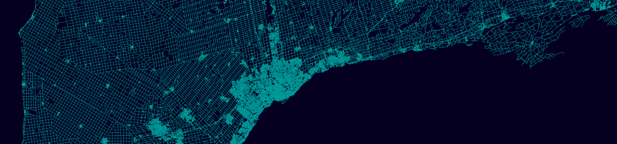
With the census values distributed throughout the country, the resulting csv file can be loaded into QGIS and symbolized by language as below, here where red equals English, blue French, and green bilingual speakers.
The patterns in overall population density are clear, with the highest density regions found in southern Ontario and Québec, and major cities like Vancouver, Calgary, Edmonton, and Winnipeg.
Official language speakers are shown to be primarily English across most provinces, transitioning to bilingual closer to the Québec border, the province where French speakers are most common. The largest densities of bilingual speakers can be seen in cosmopolitan cities like Ottawa, Montréal, and Québec city.
