All roads vector map: part 3

This is the final entry in my three part series detailing the creation of a vector map from scratch. This post covers displaying the vector tiles created in part 1 with the styling of part 2, in a JavaScript web map, here using Mapbox GL JS.

If not already active, first start a localhost instance of tileserver-gl to serve the style from part 2, by running the below command in a terminal within the directory containing the server files – config.json; road.mbtiles; and the style file.

docker run --rm -it -v $PWD:/data -p 80:80 klokantech/tileserver-gl

Connect to tileserver at localhost, and make a note of the url for the style.json listed under GL Style e.g. http://localhost/styles/road/style.json. This is the endpoint of our styled tiles, and what is needed to display them in a web map.

For the web map, I am using Mapbox’s GL JavaScript library, probably the most fully featured and simple solution for displaying vector tiles. To start, take the simple map example and copy this to a text file named index.html like below.

<!DOCTYPE html>
<html>
<head>
<meta charset="utf-8" />
<title>Display a map</title>
<meta name="viewport" content="initial-scale=1,maximum-scale=1,user-scalable=no" />
<script src="https://api.mapbox.com/mapbox-gl-js/v1.11.0/mapbox-gl.js"></script>
<link href="https://api.mapbox.com/mapbox-gl-js/v1.11.0/mapbox-gl.css" rel="stylesheet" />
<style>
    body { margin: 0; padding: 0; }
    #map { position: absolute; top: 0; bottom: 0; width: 100%; }
</style>
</head>
<body>
<div id="map"></div>
<script>
    // TO MAKE THE MAP APPEAR YOU MUST
    // ADD YOUR ACCESS TOKEN FROM
    // https://account.mapbox.com
    mapboxgl.accessToken = '<your access token here>';
    var map = new mapboxgl.Map({
        container: 'map', // container id
        style: 'mapbox://styles/mapbox/streets-v11', // stylesheet location
        center: [-74.5, 40], // starting position [lng, lat]
        zoom: 9 // starting zoom
    });
</script>

</body>
</html>

Then, simply edit the map object to refer to our own style url from tileserver-gl – the mapbox token can also be removed, this is not required when using non-Mapbox styles. So, replace the lines within the <script> tags with something like:

<!DOCTYPE html>
<html>
<head>
<meta charset="utf-8" />
<title>Display a map</title>
<meta name="viewport" content="initial-scale=1,maximum-scale=1,user-scalable=no" />
<script src="https://api.mapbox.com/mapbox-gl-js/v1.11.0/mapbox-gl.js"></script>
<link href="https://api.mapbox.com/mapbox-gl-js/v1.11.0/mapbox-gl.css" rel="stylesheet" />
<style>
    body { margin: 0; padding: 0; }
    #map { position: absolute; top: 0; bottom: 0; width: 100%; }
</style>
</head>
<body>
<div id="map"></div>
<script>
    var map = new mapboxgl.Map({
        container: 'map',
        style: 'http://localhost/styles/road/style.json',
        center: [-80.0, 50],
        zoom: 4,
        minZoom: 4,
        maxZoom: 16
    });

    // Add zoom and rotation controls to the map.
    map.addControl(new mapboxgl.NavigationControl());
</script>

</body>
</html>

This also updates the default map view with the zoom and center parameters to display Ontario when connecting to the map, and limits in min and max zoom levels to match the zoom levels present in the tiles. We can also add a control with map.addControl, in this case zoom and rotation controls.

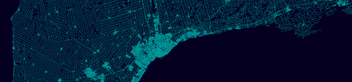
Opening index.html in a browser should give you something like below – a fully functioning web map, running off of tileserver-gl.

All roads vector map: part 2

Resuming from part 1, this post continues in outlining the steps for developing a roads web map, next discussing styling vector tiles with maputnik.

First, start a tileserver-gl instance on localhost with the roads.mbtiles database from part 1, using the –verbose parameter to display the configuration options, which we can use later:

docker run --rm -it -v $PWD:/data -p 80:80 klokantech/tileserver-gl --verbose

Next, access the tileserver frontend via a browser by connecting to localhost:8080, and click the TileJSON button to obtain a url for the served data – something like: http://localhost/data/road.json. Make note of this url.

To style the data, we can use the maputnik editor, also available to run locally via Docker, as below. Note that a previous edit of this post used the online editor, but this now blocks HTTP requests (i.e. our localhost data source) due to CORS. If we also run maputnik on localhost, this gets around the problem.

docker run --rm -it -p 8888:8888 maputnik/editor

Connect to the app at http://localhost:8888/, which will likely display a default example style, so first clear this by selecting Open from the header, and from the gallery options, Empty Style. Next, set a name and owner for the new style under the Style Settings tab.

We can now add our server data from the Data Sources tab, under Add New Source. To do this, set the source type to TileJSON, the url to your localhost url from earlier, choose a suitable ID, then hit Add Source.

The next step is to add that layer to the style with the Add Layer button of the Layers pane. Set the source ID from above, the name of the layer to style, and a layer ID (here all are simply “road”), and set the (geometry) type to line, then click Add Layer.

Note that the roads layer may be outside the current map bounds and not immediately visible, so browse to http://localhost:8888/#4/50/-80 to center the map on Ontario, where if all is well, the roads layer should be visible, with default styling options applied.

We can customize the styling of the roads layer with various options in the layers panel. For example, adjusting the min and max zoom levels the layer is displayed, the color, and the width, as below. Here, I’ve set the width to vary by zoom level, to improve visualization. This can be done by clicking the epsilon button and setting min/max values for the range: 0.1 px at zoom level 4 to 1 px at zoom levels 10+.

Also add a background layer with the same Add Layer control, and set a suitable fill color under Paint properties. Make sure to drag the new layer below roads in the layer panel, otherwise it will be drawn above it.

With this basic style complete, hit the Export button, and download the style as a JSON file. We can now create a config JSON file for tileserver-gl to use the style, based on the default config that is displayed by the –verbose option of the earlier tileserver-gl run. Create something like the below with a text editor, changing the “style” and “mbtiles” paths as needed. Save this in the same directory as your .mbtiles file as config.json.

{
  "options": {
    "paths": {
      "root": "/usr/src/app/node_modules/tileserver-gl-styles",
      "fonts": "fonts",
      "styles": "styles",
      "mbtiles": "/data"
    }
  },
  "styles": {
    "road": {
      "style": "/data/styles/mapping_on_roads.json"
    }
  },
  "data": {
    "road": {
      "mbtiles": "road.mbtiles"
    }
  }
}

Restart the tileserver-gl instance to read from the new config file, and again connect to the app at localhost. Click Viewer to generate a sample map, and check that your style file has been applied.

The next and final step will be to display the same styled vector tiles in a web map outside of tileserver, the topic of the next post.

All roads vector map: part 1

Welcome to my blog, all about mapping Ontario, Canada (and beyond) with free and open source GIS tools and data. I am starting out with a three part tutorial, which will demonstrate creating the ON roads web map from the maps page, using a range of GIS tools, including GDAL/OGR, tippecanoe, tileserverGL, maputnik, and mapbox-gl.js. As installing these libraries may not be straight forward on all operating systems, and out of scope for this blog, I suggest using Docker and running dedicated containers for each task, where applicable. QGIS is also recommended, as a general purpose method for reviewing spatial data.

We will first need some GIS data to work with. As a case study, I am using the Ontario Road Network (ORN), which may be found at the Ontario Geohub. To follow along, first download and unzip the data, selecting the ESRI Shapefile format. Optionally preview the data with QGIS, if installed.

To run the vector tile generation tool tippecanoe, we next need to transform our shapefile to the desired GeoJSON format. To do this we can use the ogr2ogr spatial data conversion tool, available as a stand alone application or with a docker image like osgeo/gdal:alpine-small-latest, as with the example below.

This command reads the road network layer from the current directory ($PWD, mounted as /mapping-on), and filters the output attributes to only retain the geometry column using SQL (-dialect & -sql), to reduce the file size. The transformed and filtered output is written to a file called road.geojson. Omit the code before ogr2ogr and adjust the file paths if installed stand alone.

docker run --rm -v $PWD:/mapping-on osgeo/gdal:alpine-small-latest ogr2ogr -dialect sqlite -sql "select geometry from Ontario_Road_Network_ORN_Road_Net_Element" /mapping-on/road.geojson /mapping-on/Ontario_Road_Network_ORN_Road_Net_Element/Ontario_Road_Network_ORN_Road_Net_Element.shp

With the roads data now transformed to GeoJSON format, we can use tippecanoe to generate vector tiles for mapping. In brief, vector tiles are a compressed and efficient method of delivering spatial data to a browser for client side styling and rendering, in contrast to the more “traditional” server side raster (image) rendering, which can be resource intensive. Tippecanoe is one of many tools that can generate vector tiles from other data sources.

The simplest way to get started with tippecanoe is again via docker, as below. This command generates an mbtiles database of vector tiles from zoom levels 4 (low) to 12 (high), and a low-zoom detail level of 10 (from a default of 12, lower is less detail). Tippecanoe will simplify, aggregate and filter the data at each zoom level to reach an optimized tile size for mapping, while aiming to retain the shape, density, and distribution of the original data.

docker run --rm -v $PWD:/mapping-on ssastbury/tippecanoe:latest -f -D10 -Z4 -z12 -o /mapping-on/road.mbtiles /mapping-on/road.geojson

With the vector tiles generated, we can now think about serving them for styling. A free and open source way to do this is with TileserverGL, a user friendly server for vector tiles. Running the klokantech/tileserver-gl docker image with default parameters as below, will search for a .mbtiles file in the current directory, and serve the tiles on port 8080 of your machine.

 docker run --rm -it -v $PWD:/data -p 8080:80 klokantech/tileserver-gl 

Point your browser to localhost:8080 and you should see tileserver up and running. Click the Inspect button to generate a basic slippy map with an interactive preview of your tiles. The next job is to apply our own custom styling to the data, which is the topic of my next post.